# Probability Distributions
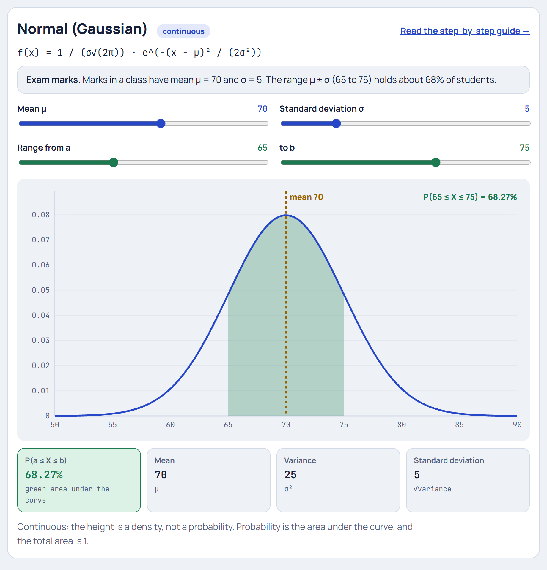
**[▶ Live demo: Distribution Explorer](https://yanshuman.github.io/cryptography/distribution/)** · [All projects](../README.md)
A **probability distribution** tells you how likely each possible outcome is. This folder explains the 10 most important distributions **step by step**. Each guide follows one real-life example all the way through, and every number is built from an earlier step. The **Distribution Explorer** lets you move the parameters and see the probabilities change.
## Contents
1. [The basics: what is a distribution?](#1-the-basics-what-is-a-distribution)
2. [The 10 distributions](#2-the-10-distributions)
3. [How they are connected](#3-how-they-are-connected)
4. [Which one should I use?](#4-which-one-should-i-use)
5. [Suggested reading order](#5-suggested-reading-order)
6. [Distribution Explorer](#6-distribution-explorer)
7. [Questions & Answers](#7-questions--answers)
---
## 1. The basics: what is a distribution?
A **random variable** X is a number decided by chance: the number of free throws made, the wait for a bus, a student's exam mark. Its **distribution** lists every value X can take and how likely each one is.
### Discrete vs continuous
| | Discrete | Continuous |
|---|---|---|
| Values | Separate counts: 0, 1, 2, … | Any value in a range: 4.73, 9.2… |
| Example | Calls per hour, rolls until a 6 | Waiting time, height, income |
| Described by | **PMF**: P(X = k), a bar for each value | **PDF**: a density curve f(x) |
| Probability of a range | **Add the bars** | **Area under the curve** |
| Probability of one exact value | Can be > 0 | Always 0, because a point has no width |
| Total | All bars add to 1 | Total area is 1 |
### Four numbers that describe any distribution
| Term | Meaning | Formula (discrete) |
|---|---|---|
| **Mean** (expected value) μ | The long-run average | Σ x · P(x) |
| **Variance** σ² | Average squared distance from the mean | Σ (x − μ)² · P(x) |
| **Standard deviation** σ | Typical distance from the mean, in the original units | √variance |
| **CDF** F(x) | Chance of getting x or less | P(X ≤ x) |
For continuous distributions, the sums become integrals.
## 2. The 10 distributions
### Discrete: counting things
| Distribution | Answers | Parameters | Mean | Variance | Running example |
|---|---|---|---|---|---|
| [**Bernoulli**](bernoulli.md) | Did one try succeed? | p | p | p(1 − p) | One free throw, p = 0.7 |
| [**Binomial**](binomial.md) | How many successes in n tries? | n, p | np | np(1 − p) | Makes out of 10 free throws |
| [**Poisson**](poisson.md) | How many events in an interval? | λ | λ | λ | Calls per hour, λ = 3 |
| [**Geometric**](geometric.md) | How many tries until the first success? | p | 1/p | (1 − p)/p² | Rolling a die until a 6 |
### Continuous: measuring things
| Distribution | Answers | Parameters | Mean | Variance | Running example |
|---|---|---|---|---|---|
| [**Uniform**](uniform.md) | Every value in a range equally likely | a, b | (a + b)/2 | (b − a)²/12 | Waiting for a bus, 0 to 10 min |
| [**Normal (Gaussian)**](normal.md) | Many small effects added together | μ, σ | μ | σ² | Exam marks, μ = 70, σ = 5 |
| [**Exponential**](exponential.md) | Waiting time until the next event | λ | 1/λ | 1/λ² | Time to the next call, λ = 3/hour |
| [**Log-normal**](lognormal.md) | Many small effects multiplied together | μ, σ (of ln X) | e^(μ+σ²/2) | (e^σ² − 1)e^(2μ+σ²) | Monthly income |
| [**Chi-square**](chi-square.md) | Is the gap between observed and expected just luck? | k | k | 2k | Is this die fair? |
| [**Student's t**](t-distribution.md) | A small-sample mean when σ is unknown | ν | 0 | ν/(ν − 2) | Testing 6 batteries |
Each guide contains:
- a picture of the distribution with the example shaded
- a step-by-step build-up, from the real-life picture to the formula, explaining where every piece comes from
- worked numbers for the mean, variance and probabilities
- a summary table, where it's used, and a one-line answer for exams
## 3. How they are connected
The distributions form one family. Each arrow shows how one turns into another:
```
repeat n times, count successes
Bernoulli(p) ─────────────────────────────────────► Binomial(n, p)
│ │ │
│ repeat until the n large, │ │ n large
│ first success p tiny, │ │ (Central Limit
▼ np = λ ▼ ▼ Theorem)
Geometric(p) Poisson(λ) Normal(μ, σ)
┆ │ │ │ │
┆ continuous twin gaps between │ │ │ │
┆ (both memoryless) events │ │ │ │
▼ ▼ │ │ │
Exponential(λ) ◄───────────────────────────────────────┘ │ │ │
│ │ │
X = e^(normal) ◄─────────────────────────┘ │ │
Log-normal │ │
│ │
sum of k squared standard normals ◄──────────┘ │
Chi-square(k) │
│ │
└──► normal ÷ √(chi-square / ν) ◄─────────┘
Student's t(ν)
Uniform(0, 1): the seed. Computers turn uniform random numbers
into every other distribution above (inverse transform sampling).
```
In words:
- **Bernoulli** is the atom. **Binomial** counts Bernoulli successes, and **Geometric** waits for the first one.
- **Binomial → Poisson** when there are many trials with a tiny chance each.
- **Poisson ↔ Exponential:** counts of events vs the gaps between them.
- **Geometric ↔ Exponential:** the discrete and continuous "waiting time" distributions, both memoryless.
- **Binomial and Poisson → Normal** for large n or λ: the Central Limit Theorem.
- **Normal → Log-normal** (take e^X), **→ Chi-square** (square and add), and **→ t** (divide by an estimated spread).
## 4. Which one should I use?
```
Is the outcome a COUNT (0, 1, 2, …)?
├── YES
│ ├── Just one try, yes/no? → Bernoulli
│ ├── Fixed number of tries, count the successes? → Binomial
│ ├── Count events in a time or space interval? → Poisson
│ └── Count tries until the first success? → Geometric
│
└── NO, it's a MEASUREMENT (any value)
├── Every value in a range equally likely? → Uniform
├── Waiting time until a random event? → Exponential
├── Sum of many small effects, symmetric? → Normal
├── Positive, grows by percentages, long tail? → Log-normal
└── It's a TEST STATISTIC
├── Comparing observed vs expected counts? → Chi-square
└── Small-sample mean, σ unknown? → Student's t
```
## 5. Suggested reading order
The examples are linked, so this order builds each idea on the last:
1. [Bernoulli](bernoulli.md): one free throw
2. [Binomial](binomial.md): 10 free throws (Bernoulli repeated)
3. [Geometric](geometric.md): rolling until a 6 (Bernoulli until the first success)
4. [Poisson](poisson.md): calls per hour (Binomial with tiny pieces)
5. [Exponential](exponential.md): time between those calls
6. [Uniform](uniform.md): waiting for a bus
7. [Normal](normal.md): exam marks
8. [Log-normal](lognormal.md): incomes (Normal on a log scale)
9. [Chi-square](chi-square.md): is the die fair? (squared normals)
10. [Student's t](t-distribution.md): testing 6 batteries (Normal with an estimated σ)
## 6. Distribution Explorer
[`index.html`](index.html) is a single-page app:
- **Pick any of the 10 distributions.** Each starts with the example from its guide.
- **Move the parameters** (n, p, λ, μ, σ, k, ν) with sliders and watch the shape change.
- **Drag the green range** (a to b) to see P(a ≤ X ≤ b) as shaded bars or area.
- **Live stats:** the mean (also marked on the chart), variance, standard deviation, and the formula.
- **Student's t** is drawn against a dashed standard normal, so you can see the heavier tails.
- **Direct links:** add `#normal`, `#binomial`, `#poisson` and so on to the URL to open a specific distribution.
**How to run:** no installation needed. Double-click `index.html`, run `start index.html` in this folder, or use the [live demo](https://yanshuman.github.io/cryptography/distribution/).
## 7. Questions & Answers
What's the difference between a PMF and a PDF?
A **PMF** (probability mass function) is for discrete variables: P(X = k) is an actual probability, drawn as a bar. A **PDF** (probability density function) is for continuous variables: f(x) is a *density*, and only the **area** under it between two values is a probability. That's why a PDF can be taller than 1, like the Exponential's height of 3 at t = 0.
Why is the probability of one exact value 0 for continuous variables?
Probability is area, and a single point has zero width, so zero area. The chance a bus wait is *exactly* 5.000000… minutes is 0, but the chance it's between 4.9 and 5.1 minutes is 0.2/10 = 2%.
Why does the Normal distribution appear everywhere?
Because of the **Central Limit Theorem**: when a quantity is the **sum of many small independent effects**, its distribution approaches a bell curve, whatever the individual effects look like. Heights, measurement errors and exam marks are all such sums. See [Normal, Step 2](normal.md#step-2-why-does-a-bell-shape-appear).
Binomial or Poisson: how do I choose?
Use the **Binomial** when there's a fixed number of tries n and you count successes (7 out of 10 shots). Use the **Poisson** when events happen at a rate in time or space with no fixed number of tries (calls per hour). If n is large and p is small, the two give almost the same answers with λ = np.
What does "memoryless" mean?
Past waiting doesn't change future waiting. After 10 rolls with no 6, the chance of needing more than 3 more rolls is the same as from scratch. Only the **Geometric** (discrete) and **Exponential** (continuous) distributions have this property. Believing otherwise ("I'm due a 6") is the gambler's fallacy.
Why divide by n − 1 instead of n for a sample's standard deviation?
The sample mean is calculated from the same data, so the data sits closer to it than to the true mean, and dividing by n would underestimate the spread. Dividing by n − 1 corrects this. The "1" is the degree of freedom used up by estimating the mean. See [Student's t, Step 6](t-distribution.md#step-6-degrees-of-freedom-the-tails-shrink-as-the-sample-grows).
What are "degrees of freedom"?
The number of values that are free to vary once constraints are applied. With 6 die counts that must total 60, only 5 are free (the 6th is forced), so k = 5. With a sample of 6 used to estimate its own mean, ν = 5. More degrees of freedom means more information, and the Chi-square and t distributions change shape accordingly.
Mean, median or mode: which "average" should I report?
For symmetric distributions (Normal, Uniform, t) they're all equal. For **right-skewed** ones (Log-normal, Exponential, Poisson with small λ), mode < median < mean, because a long right tail pulls the mean up. For incomes and house prices, the **median** better describes a typical value. See [Log-normal, Step 6](lognormal.md#step-6-mode-median-and-mean-three-different-centres).
How do computers generate random numbers from these distributions?
They start from a **Uniform(0, 1)** random number U and transform it. For example, −ln(U)/λ is Exponential, and the Box–Muller formula turns two uniforms into a Normal. See [Uniform, Step 8](uniform.md#step-8-why-computers-love-the-uniform).
---
### Files
```
distribution/
├── README.md # This overview
├── index.html # Distribution Explorer
├── bernoulli.md # One try: success or failure
├── binomial.md # Successes in n tries
├── poisson.md # Events in an interval
├── geometric.md # Tries until the first success
├── uniform.md # Every value equally likely
├── normal.md # The bell curve (Gaussian)
├── exponential.md # Waiting time between events
├── lognormal.md # Multiplicative growth
├── chi-square.md # Observed vs expected counts
├── t-distribution.md # Small-sample means
└── images/ # One picture per distribution (from the Explorer)
```